Task 3

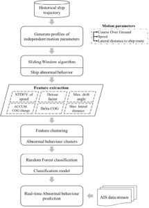
• standard deviation of speed;
• detour factor;
• maximum drift angle;
• accumulative COG change;
• delta COG;
• maximum lateral distance.

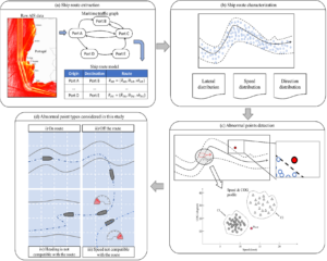
1. Ship route extraction that groups the ship trajectories according to corresponding motion patterns;
2. Ship route characterisation that constructs a normalcy model for ship routes based on the analysis of ship trajectory clusters in terms of lateral distribution along the ship route, speed distribution and Course Over Ground (COG) distribution;
3. Ship abnormal points detection using the normalcy model.

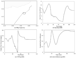
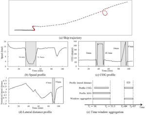
Ship abnormal behaviour is detected when the speed, COG and lateral distance considerably deviate from other ships within the same route. Figure 3(a) shows a ship trajectory while Figure 3(b), (c) and (d) depict the profiles of three independent motion parameters, namely speed, COG and lateral distance to ship route centreline, respectively. It is seen that the ship trajectory, Figure 3(a), exhibits a circular behaviour, and the profiles in Figure 3(b), (c) and (d) show abnormality in the motion parameters during the circular behaviour. Specifically, the speed profile in Figure 3(b) shows that the ship’s speed decreases significantly during the circular behaviour. The COG profile and lateral distance profile show that the ship’s course deviates and lateral distance to the route centreline varies significantly during the circular behaviour, respectively. Therefore, the abnormality in the motion parameter profiles enables to detect the time interval when the ship is exhibiting abnormal behaviour that requires further investigation.

The main goal of detecting ship abnormal behaviour is looking into motion profiles at each part of the original trajectory locally and capturing any abnormality which has occurred in trajectory behaviour. For this purpose, a Sliding Window approach is applied to analyse ship motion data by moving over various profiles (e.g., speed, COG and lateral distance) simultaneously, and generating several sub-profiles in each window. The window is flagged as abnormal by comparing the calculated motion parameters within each window with pre-defined thresholds. If the time interval between two flagged abnormal windows is less than a time threshold (in this study it is 30 minutes), these windows are aggregated into a single time interval of ship abnormal behaviour. Otherwise, the abnormal behaviour is considered to be separated and a new time interval is formed for the subsequent flagged windows.

The main idea of ship abnormal behaviour detection is first to scan the points in positive order for initial detection of possible abnormal points, and then aggregate the abnormal points to form ship abnormal behaviour in a certain time interval. The evaluation of each point is based on the speed, COG and lateral distance distributions compared with the neighbour historical AIS data. An illustration of the key elements of the ship abnormal behaviour detection approach is presented in Figure 4.

Figure 4(a) shows a ship trajectory with two identified abnormal behaviours. In Figure 4(b), it is observed that the ship experiences a significant decrease in speed between 34 minutes and 51.3 minutes. In Figure 4(c), it is observed that abnormal COG values are present in time intervals [36 min, 48.3 min] and [84 min, 97 min]. Additionally, Figure 4(d) reveals that the ship navigates offroute for 87 min and 93 min, as the normalised lateral distance falls below -1. The sliding window technique allows for the detection of abnormal ship behaviour by analysing motion parameter sub-profiles over small-time intervals. By combining the abnormal sub-profiles into time intervals of abnormal behaviour, as a result, the proposed method effectively identifies the two instances of abnormal ship behaviour occurring during time intervals [34 min, 51.3 min] and [84 min, 97 min], respectively. By analysing the sub-profiles generated from the sliding window approach, abnormal values for speed, COG, and lateral distance are identified and used to form time intervals of abnormal behaviour. These results demonstrate the potential of the proposed method in identifying abnormal ship behaviour based on multiple motion parameters.

Ship trajectory classification is a process of creating a model that can match the motion pattern of an object to a specific label based on certain decision criteria. Though several trajectory classification solutions have been proposed and applied in many domains, less focus has been given to the maritime domain. Available applications have been used in classifying a vessel’s type, e.g., [2] and [3], characterising shipping operation areas, e.g., [4], and search and rescue operations, e.g., [5], [6], based on its trajectory. Several features that are capable of capturing the observed ship abnormal behaviour can be considered to create a proper classification model. The proposed features include:

1. Standard deviation of speed;
2. Detour factor;
3. Drift angle;
4. COG change;
5. Accumulative of COG change;
6. Normalised maximum lateral distance.

Standard deviation of speed

Ships when engaged in navigation tend to maintain a constant speed without any significant change. The standard deviation can reveal whether the speed is constant or not during a ship’s trajectory. A standard deviation of speed close to zero indicates the steadiness of the speed.

Detour Factor

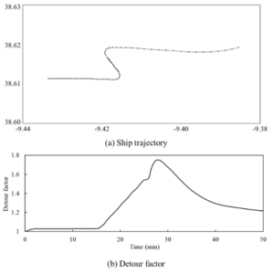
Detour Factor (DF) is a widely used feature in various areas of transportation. A detour often happens when the ships make a U-turn or circular movements. It is employed to quantify the degree of detour as an anomalous feature. As shown in Equation below and Figure 5(a), for each individual position in the ship trajectory, the DF is defined as the ratio of the trajectory length to the geodesic distance from its start point to the current position:

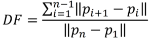
where ‖∙‖ represents the distance between two points in a ship trajectory.

Maximum drift angle

The drift angle is the angle between the axis of a ship when turning and the tangent to the path on which it is turning. It can be inferred from the difference between the COG and the heading of the vessel. The COG represents the actual direction the vessel has along its path, while the heading represents the direction of the vessel’s bow. When manoeuvring ships, mariners usually pay great attention to the rate at which the heading changes, but the direction in which the ship actually moves may differ from the direction in which she is heading. Therefore, an excessive drift angle is indicative of the abnormal ship behaviour at the turning moments.

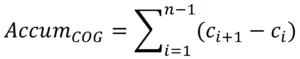
Accumulative COG change

The accumulative COG change refers to the total change in a ship’s COG over a ship trajectory. It is calculated by summing up the changes in COG between each consecutive points along the ship trajectory, as shown in Equation below. A high accumulative COG change over a period of time may indicate that the ship is experiencing abnormal or unexpected behaviour, such as U-turn, double U-turn or circular behaviours.

Delta COG

The delta COG is defined as the absolute value of the difference between Course Over Ground at the start and end points of a ship trajectory. In terms of abnormal behaviour detection, delta COG can be used as a feature to detect abnormal behaviour of a ship as it represents the deviation from a straight-line course and indicates that the ship did not maintain a constant heading during a voyage leg.

Maximum lateral distance

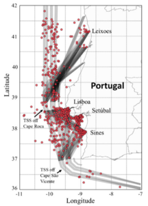
In the context of maritime traffic, ships navigate from one place to another using the most effective path, and therefore grouping similar ship trajectories into clusters provides an overview of the general traffic patterns. This normalcy representation supports anomaly detection of ship trajectories that deviate from the route behaviour. As the centreline and the route boundary of the ship routes are represented by a set of geographical points, if the ship position is located inside the ship routes, then the ship is labelled as within-route. Ship off-route behaviour may be caused by several reasons: the ship may deviate from the route to avoid other ships or turn towards the destination (or next waypoint) too soon or too late.

In the next step, a classification model is trained based on the features extracted from the clusters formed through a density-based clustering method, which groups similar patterns of ship abnormal behaviours. Clustering is a process of partitioning data into meaningful groups of objects with similar features in the feature space, and density-based clustering methods, such as Density-Based Spatial Clustering of Applications with Noise (DBSCAN), is particularly useful for datasets with varying densities and noise.

After clustering the extracted features of historical abnormal behaviours, each trajectory and feature vector are labelled with its corresponding cluster number which represents a specific behaviour pattern. Then, the labelled feature vectors are used to train a multi-class Random Forest (RF) classification model due to its high-performance and less prone to overfitting characteristics [5], which has been already adopted in the maritime domain [6], [7]. The RF classification model works by creating an ensemble of decision trees and then combining their outputs to make a final classification decision. Then, the trained multi-class classification model can be used to predict the abnormal behaviour of new ship trajectories.

Five hyper-parameters are considered in the proposed prediction model:

1. The maximum depth of a tree (max depth).
2. The minimum number of data entries required to split a node (min samples split).
3. The minimum number of data entries required to be at a leaf node (min samples leaf).
4. The number of decision trees contained in the forest (n estimators).
5. The number of features to consider when finding the best split of a node in each decision tree (max features).

Grid search is a common method to determine the optimal hyperparameters for a Random Forest Classification model. The general idea is to define a range of values for each hyperparameter and then train and evaluate the model using every combination of hyperparameters within those ranges. The hyperparameters with the best performance are then selected as the optimal hyperparameters.

As a first evaluation of the ship abnormal behaviour detection algorithm, a discriminant validity test is performed. This test is used to evaluate whether the model appropriately distinguishes situations representing ship abnormal behaviour. For the discriminant validity test, four abnormal behaviours in ship trajectories are selected, and the time durations of abnormal behaviours are detected based on the proposed ship abnormal behaviour detection algorithm. The features extracted for the abnormal behaviours are listed in Table 1, and the last column indicates the type of ship abnormal behaviour.

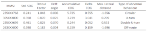
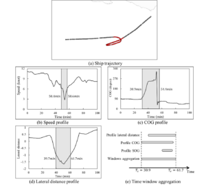
Figure 7(a) illustrates the case of a ship having a “Circular” behaviour. Each ship abnormal behaviour detection is described on five panels of the figure. The top panel shows the ship trajectories with abnormal behaviour, where grey colour indicates normal behaviour and red colour indicates abnormal behaviour. The panels “bcd” show the speed profile, COG profile and normalized lateral distance profile, respectively. Panel “e” shows the time window aggregation to form the time duration of the ship abnormal behaviour.

As shown in Figure 7, the ship’s speed suddenly decreased in the time interval [50.4𝑚𝑖𝑛, 58.6𝑚𝑖𝑛] and the COG values are not within the normal range of the ship route (range of 60° to 90°), indicating that the ship is not following its designated route between time interval [30.9𝑚𝑖𝑛, 54.4𝑚𝑖𝑛]. Additionally, the ship deviated from its route between time intervals [39.7𝑚𝑖𝑛, 61.7𝑚𝑖𝑛] with the lateral distance being less than -1. Therefore, the duration of the abnormal behaviour is [30.9𝑚𝑖𝑛, 61.7𝑚𝑖𝑛].

The proposed method can identify the time interval of abnormal behaviour within ship trajectories by analysing speed, COG and lateral distance profiles of ship trajectories based on the sliding window method. Once the ship abnormal behaviours are detected, a set of features are calculated to further characterise the behaviour. The DBSCAN algorithm is then applied to cluster the ship abnormal behaviour based on the extracted features, which allows for the identification of typical patterns of abnormal behaviour. Four clusters corresponding to the four types of ship abnormal behaviours were recognised by the DBSCAN algorithm:

• Cluster 1 reflects the circular abnormal behaviour type, includes the trajectories where the speed is decreasing, the accumulative COG is around 2𝜋 while the delta COG is small.
• Cluster 2 exhibits a U-turn ship behaviour with accumulative COG and delta COG around 𝜋.
• Cluster 3 is characterised by ship behaviour with large detour factors, and both accumulative COG and delta COG remain small, associated with the double U-turn behaviour.
• Cluster 4 has the maximum lateral distance which exceeds 1 or -1, corresponding to an off-route abnormal behaviour type.

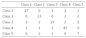
To evaluate the performance of the Random Forest classification model trained on the features extracted from ship abnormal behaviours, a confusion matrix is generated based on the test data set. The test dataset (25% of the whole dataset) is a subset of the original dataset that is not used during training, but to evaluate the model’s ability to generalise to new data. A confusion matrix summarises the performance of a classification model in terms of the number of correctly and incorrectly classified instances in each class. As shown in Table 2, the rows and columns of the matrix represent the actual class labels and the predicted class labels, respectively. The diagonal elements of the matrix represent the number of correct predictions, while off-diagonal elements represent incorrect predictions. According to the confusion matrix, the multi-class classification model performs well with most of the diagonal elements being higher than off-diagonal elements. However, there are some incorrect classification cases, especially for Class 3, where there are 8 false negatives and 5 false positives. This could happen if the features of these instances are similar to the features of other classes, which makes it difficult for the classification model to distinguish them from other classes. Class 5 represents the noise data points that were not clustered with any of the other classes in the feature space by the DBSCAN algorithm. These ship abnormal behaviours do not have a clear pattern or similarity with other classes, and therefore, it is expected to have a lower classification accuracy, compared with the other classes. In other words, the multi-class classifier may not have learned a clear decision boundary for Class 5 since it contains data points (represent features of ship abnormal behaviours) close to data points in the other classes.

Machine Learning models are often black boxes that make their interpretation difficult, however, Explainable Machine Learning (EML) techniques provide some insight into their inner workings. One popular EML method is SHAP (SHapley Additive exPlanations) values, which uses cooperative game theory to explain how each feature affects the model’s output. SHAP values are a technique used to explain the contribution or the importance of each feature on the prediction of the classification model, and it can be used to increase the transparency and interpretability of machine learning models.

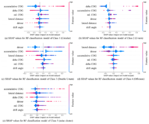
Figure 8 shows the SHAP values for the Random Forest classification models. In the figure, the features are ordered by their effect on corresponding predictions, and the effect of higher and lower values of each feature on the classification result can also be observed. The horizontal axis represents the SHAP value, and the dots on the plot represent a single observation while the colour of the point indicates that the observation has a higher or a lower value of the features.

Based on the SHAP values analysis in Figure 8, it can be observed that the features have different contributions to the classification of different classes. Please note:

• the feature accumulative COG has the most significant contribution to Class 1;
• the feature delta COG has the most significant contribution to Class 2;
• the feature detour factor has the most significant contribution to Class 3;
• the feature maximum lateral distance has the most significant contribution to Class 4.

As shown in Figure 8 (a), it is seen that the higher values of accumulative COG have a positive impact on the prediction of Class 1; however, for Class 3, higher values of accumulative COG have a negative impact (Figure 8 (c)). In addition, detour factors have a positive impact on the prediction of Class 3, while lower values have a positive impact on the prediction of Class 4. Regarding the feature of maximum lateral distance, it is seen that the contribution of maximum lateral distance is relatively small for Class 1, Class 2 and Class 3. In contrast, for Class 4, the feature has a significant contribution to the prediction, with higher values showing a dominant effect (the SHAP values of higher values located in the range of [0.4,0.6]), and higher values (red dots) and lower values (blue dots) are clearly separated. Therefore, it can be concluded that the feature of maximum lateral distance is dominant in predicting Class 4.

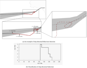
The RF classification model is now applied to predict the ship abnormal behaviour in a ship trajectory. In Figure 9(a), the grey markers represent the normal ship behaviour while the red markers highlight the abnormal behaviour, and Figure 9 (b) shows the classification of ship behaviour. It should be mentioned that Class zero represents normal behaviour.

As shown in Figure 9 (a), the ship is first assigned to the ship route based on its positional information, moving eastward with speed and COG in accordance with the ship route. At 𝑡 = 128.3𝑚𝑖𝑛, the ship starts heading south-eastward and begins to deviate from the ship route, resulting in the RF classification model assigning it as Class 5 during the time [128.3𝑚𝑖𝑛, 137.6𝑚𝑖𝑛]. Subsequently, the ship’s deviation from the ship route is classified as Class 4 representing an off-route abnormal behaviour between 𝑡 = 137.6𝑚𝑖𝑛 and 176.1𝑚𝑖𝑛. At 𝑡 = 176.1𝑚𝑖𝑛, the ship begins turning starboard side, and at 𝑡 = 186.3𝑚𝑖𝑛 the ship is classified as Class 2 mainly due to the delta COG of ship trajectory during this time interval being 163.4°. The ship continuously turns starboard side and is then classified as Class 1, indicating circular behaviour. After exhibiting various abnormal behaviours classified by the RF classification model, the ship finally returns to the intended ship route and proceeds towards the port of Lisboa.